Car Detection using OpenCV and Python within 5 minutes!

Today, you’ll explore an advanced vehicle detection system and classification project built with OpenCV in this article. The article will guide you in using the YOLOv3 model with OpenCV-python. Open-CV is a Python real-time computer vision library. Let’s start with the basics here first.

The Concept of Detecting Moving Objects in Videos

Object detection is an enthralling area of computer vision. When we’re dealing with video data, it takes on a whole new level. The intricacy increases, but so do the rewards! Using object detection techniques, we can do extremely helpful high-value jobs such as surveillance, traffic control, criminal fighting, etc.

Here’s an animated GIF to demonstrate the concept: Counting the number of objects, determining the relative size of the items, and determining the relative distance between the objects are all sub-tasks in object detection. These sub-tasks are crucial since they help solve some of the most difficult real-world challenges.

Let’s look at some intriguing object detection use cases in real-world applications. Nowadays, video object detection is being used in a variety of sectors. Video surveillance, sports broadcasting, and robot navigation are among the applications. The good news is that the options are limitless regarding future use cases for video object detection and tracking. Here are some of the most fascinating applications:

• Counting the crowd
• Detection and recognition of car license plates (as discussed in the article)
• Sports ball tracking
• Robotics
• Traffic management

What Exactly Is YOLO?

YOLO is an acronym that stands for You Only Look Once. It is an object recognition algorithm that operates in real-time. It is capable of classifying and localizing several objects in a single frame. Because of its smaller network topology, YOLO is an extremely quick and accurate algorithm.

How Does YOLO Function?

YOLO mostly employs these strategies.

Residual Blocks

It essentially splits an image into NxN grids.

Regression using Bounding Boxes

The model receives one grid cell at a time. Then YOLO calculates the likelihood that the cell has a specific class, and the class with the highest probability is chosen.

IOU Or Intersection Over Union

IOU is a statistic that examines the intersection of the predicted and actual bounding boxes. A Non-max suppression technique is used to eliminate the very close bounding boxes by executing the IoU with the one with the highest-class probability among them.

The Architecture Of YOLO

The YOLO network comprises 24 convolutional layers that are followed by two fully linked layers. The convolutional layers are trained on the ImageNet classification algorithm at half the resolution (224 224 input picture) before being double-trained for detection.

• The several layers minimize the feature set from previous layers, alternate 1 1 reduction layer, and 33 convolutional layers.
• The final four layers are added to train the network to detect objects.
• The last layer forecasts the object class and bounding box probabilities.
• To interact with YOLO directly, we’ll use OpenCV’s DNN module. DNN is an abbreviation for Deep Neural Network. OpenCV includes a function for running DNN algorithms.

Vehicle Detection System And Classification Project Using OpenCV

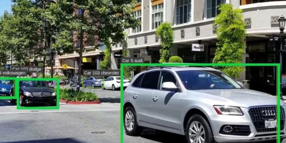
In this project, we will detect and classify cars, HMV (Heavy Motor Vehicle), and LMV (Light Motor Vehicle), on the road, as well as count the number of cars on the road. The data will be saved to examine various automobiles on the road. To complete this project, we will develop two programs.

The first will be a car detection tracker that uses OpenCV to keep track of every identified car on the road, and the second will be the primary detection software. Prerequisites for the OpenCV Vehicle Detection System and Classification Project

Python - version 3.x (We used python 3.8.8 in this project) OpenCV - version 4.4.0

DNN models should be executed on GPU whenever possible.

Numpy – 1.20.3 Pre-trained model weights and Config Files for YOLOv3.

Creating Python OpenCV Code for Vehicle Detection System and Classification In 5 Minutes You should download the OpenCV car detection and classification source code if you haven’t already.

Tracker

The tracker uses the Euclidean distance to maintain track of an item. It computes the distance between two center points of an object in the current frame and the previous frame, and if the distance is smaller than the threshold distance, it certifies that the object in the previous frame is the same in the present frame.

Import math # Get center point of new object for rect in objects_rect: x, y, w, h, index = rect cx = (x + x + w) // 2 cy = (y + y + h) // 2 # Find out if that object was detected already same_object_detected = False for id, pt in self.center_points.items(): dist = math.hypot(cx - pt[0], cy - pt[1]) if dist < 25: self.center_points[id] = (cx, cy) # print(self.center_points) objects_bbs_ids.append([x, y, w, h, id, index]) same_object_detected = True break The Euclidean distance is returned via the math.hypot() method. If the distance is less than 25, the item is the same as in the previous frame.

Counter for Cars

Steps for Detection and Classification of Cars Using OpenCV

1. Import the relevant packages and start the network.
2. Retrieve frames from a video file.
3. Run the detection after pre-processing the frame.
4. Perform post-processing on the output data.
5. Count and track all cars on the route.
6. Save the completed data as a CSV file.

Step #1 – Importing Relevant Packages And Initializing The Network

import cv2 import csv import collections import numpy as np from tracker import *

Initialize Tracker

tracker = EuclideanDistTracker()

Detection confidence threshold

confThreshold =0.1 nmsThreshold= 0.2

First, we import all of the project’s required packages. Then, from the tracker program, we initialize the EuclideanDistTracker() object and set the object to “tracker.” confThreshold and nmsThreshold are the detection and suppression minimal confidence score thresholds, respectively.

# Middle cross line position middle_line_position = 225 up_line_position = middle_line_position - 15 down_line_position = middle_line_position + 15

You need to modify the middle_line_position according to what your need is.

Store Coco Names in a list

classesFile = "coco.names" classNames = open(classesFile).read().strip().split('\n') print(classNames) print(len(classNames)) The Output

Model Files

modelConfiguration = 'yolov3-320.cfg' modelWeights = 'yolov3-320.weights'

configure the network model

Configure the network backend

net.setPreferableBackend(cv2.dnn.DNN_BACKEND_CUDA) net.setPreferableTarget(cv2.dnn.DNN_TARGET_CUDA)

Define a random color for each class

np.random.seed(42) colors = np.random.randint(0, 255, size=(len(classNames), 3), dtype='uint8')

Step # 2 – Reading The frames From The Video files

• Cap.read() reads each frame from the capture object after reading the video file using the video capture object.
• We cut our frame in half by using cv2.reshape().
• The crossing lines are then drawn in the frame using the cv2.line() function.

• Finally, we displayed the generated image using the cv2.imshow() function.

Initialize the video capture object

cap = cv2.VideoCapture('video.mp4') def realTime(): while True: success, img = cap.read() img = cv2.resize(img,(0,0),None,0.5,0.5) ih, iw, channels = img.shape # Draw the crossing lines cv2.line(img, (0, middle_line_position), (iw, middle_line_position), (255, 0, 255), 1) cv2.line(img, (0, up_line_position), (iw, up_line_position), (0, 0, 255), 1) cv2.line(img, (0, down_line_position), (iw, down_line_position), (0, 0, 255), 1) # Show the frames cv2.imshow('Output', img) if name == 'main': realTime()

Step #3 – Pre-Processing Frames And Running Detection

• Our YOLO version accepts 320320 image objects as input. The network’s input is a blob object. The function dnn.blobFromImage() accepts an image as input and returns a blob object that has been shrunk and normalized.
• The image is fed onto the network using the net. forward(). And it produces a result.
• Finally, we invoke our custom postProcess() function to post-process the output.

input_size = 320 blob = cv2.dnn.blobFromImage(img, 1 / 255, (input_size, input_size), [0, 0, 0], 1, crop=False) # Set the input of the network net.setInput(blob) layersNames = net.getLayerNames() outputNames = [(layersNames[i[0] - 1]) for i in net.getUnconnectedOutLayers()] # Feed data to the network outputs = net.forward(outputNames) # Find the objects from the network output postProcess(outputs,img)

Step #4 – Post-Processing Output

The forward network output has three outputs. Each output object is an 85-length vector.

• 4 times the bounding box (centerX, centerY, width, height)
• 1 confidence box
• 80x class assurance
• Let’s start by defining our post-processing function.

detected_classNames = [] def postProcess(outputs,img): global detected_classNames height, width = img.shape[:2] boxes = [] classIds = [] confidence_scores = [] detection = [] for output in outputs: for det in output: scores = det[5:] classId = np.argmax(scores) confidence = scores[classId] if classId in required_class_index: if confidence > confThreshold: # print(classId) w,h = int(det[2]width) , int(det[3]height) x,y = int((det[0]width)-w/2) , int((det[1]height)-h/2) boxes.append([x,y,w,h]) classIds.append(classId) confidence_scores.append(float(confidence))

Step #5 – Counting All The Tracked Cars On The Road

• After receiving all of the detections, we use the tracker object to keep track of those things. The tracker.update() function maintains track of all identified objects and updates their positions.
• The custom function Count vehicle counts the number of vehicles that have passed through the road.

• The count_vehicle Feature

• Creating two empty lists (temporary ones) for storing the car IDs entering the entry crossing line.

• To count four car classes in the up and down routes are Up_list and down_list

Function for counting vehicle

def count_vehicle(box_id): x, y, w, h, id, index = box_id # Find the center of the rectangle for detection center = find_center(x, y, w, h) ix, iy = center

• The center point of a rectangle box is returned through the find_center function.

#Find the current position of the vehicle if (iy > up_line_position) and (iy < middle_line_position): if id not in temp_up_list: temp_up_list.append(id) elif iy < down_line_position and iy > middle_line_position: if id not in temp_down_list: temp_down_list.append(id) elif iy < up_line_position: if id in temp_down_list: temp_down_list.remove(id) up_list[index] = up_list[index]+1 elif iy > down_line_position: if id in temp_up_list: temp_up_list.remove(id) down_list[index] = down_list[index] + 1

Step #6 – Saving The Final Data

• We opened a new file data.csv, with write permission only using the open function.
• Then we write three rows: the first with class names and directions, the second with up and down route counts, and the third with both.
• The writerow() function saves a row of data to a file.

#Write the car counting information in a file and save it with open("data.csv", 'w') as f1: cwriter = csv.writer(f1) cwriter.writerow(['Direction', 'car', 'motorbike', 'bus', 'truck']) up_list.insert(0, "Up") down_list.insert(0, "Down") cwriter.writerow(up_list) cwriter.writerow(down_list) f1.close()

Conclusion

Car detection with OpenCV and Python is more than just a simple coding project. It demonstrates how computer vision can solve real-world challenges through accurate vehicle detection, tracking, and analysis. With tools like YOLOv3 and OpenCV, businesses can create smarter traffic systems, improve surveillance, and unlock valuable operational insights from video data. As AI adoption accelerates, investing in scalable car detection solutions can help organizations stay ahead with faster, safer, and more intelligent decision-making.