Linear Regression with a Practical Application

For a layman, Linear Regression is as simple as a statistical method that uses a linear equation to show a relationship between two variables. In short, it is used to find the line of the best fit. At the conjunction of statistics and machine learning, linear regression is the problem of estimating the parameters (slope and y-intercept) of a linear equation, and then finding the line that best fits the data. The best fitting line is the one that minimizes the sum of the squared distances between the points on the line and the line itself.

To make it more understandable, let’s look at the image below.

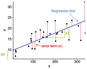
The blue line that we can see in the image above is the regression line or the line of the best fit between those black points on the graph. The red line attached to each black point is the distance (error) of that point from the line of best fit. The bigger the red line, the larger the error.

So what is the goal of linear regression?

The goal is to minimize the sum of all squared errors of all the data points.

We will try to reach our goal with the help of a practical implementation here.

Implementation:

We will implement simple linear regression for one variable to predict profits for a food truck. Suppose we are the CEO of a restaurant franchise and are considering different cities for opening a new outlet. The chain already has trucks in various cities and we have data for profits and populations from the cities. We would like to use this data to help us select which city to expand to next.

We will start by loading the dataset:

Dataset Link: https://drive.google.com/file/d/1FAIDyKWSC1BCcCayRYlhqYWNJvcOViMs/view?usp=sharing

from numpy import *
data = np.loadtxt(os.path.join('', 'ex1data.txt'), delimiter=',')
X, Y = data[:, 0], data[:, 1]

Now that we have loaded the data, let’s continue with visualising and observing how does the data look like:

pyplot.plot(X, Y, 'ro', ms=10, mec='k')
pyplot.ylabel('Profit in $10,000')
pyplot.xlabel('Population of City in 10,000s')

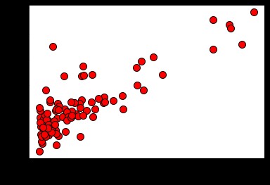
We have visualised the data, now we will progress towards our main goal: minimising the squared error, but first let us see how we will calculate the squared error?

Let’s start with the basics i.e. equation of a straight line:

Y = mX + C

We can also write it as a function of h, where h is our hypothesis.

h_θ (x) = θ_1+ θ_2 (x)

Where and are parameters to find to get the best fit and minimize the cost function, that will be coming soon below.

h(x) will be our predicted value and Y will be our actual value. Now the sum of our squared error will look something like this. This will be known as the Cost Function J(.

J(θ) =  1/2m ∑_(i=1)^m 〖(h_θ (x^((i)))-y^((i)J(θ) =  1/2m ∑_(i=1)^m 〖(h_θ (x^((i)))-y^((i)))〗^2))〗^2

Now that we have the cost function, we have to minimize it. How do you find the minimal value of a function? Yes, you guessed it right! By taking out the derivative! We will calculate the derivative with respect to both of the parameters.

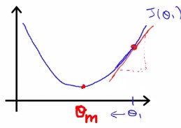
One way to do this is to use the batch gradient descent algorithm. In batch gradient descent, you try to move to the point where the slope is 0. At each iteration, we can calculate the gradient, and keep in the same direction where it is decreasing and vice versa if it is increasing.

θ_(0 )= θ_(0 )  - α 1/m ∑_(i=1)^m 〖(h_θ (x^((i)))-y^((i)))〗^
θ_(1 )= θ_(1 )  - α 1/m ∑_(i=1)^m 〖(h_θ (x^((i)))-y^((i)))x^((i))〗^

With each step of gradient descent, our parameters and come closer to the optimal values that will achieve the lowest cost J(θ).

Now that we have the theoretical knowledge, we will now write the actual code.

We will start with implementing .

def predict(x, theta0, theta1):
   '''
   Calculates the hypothesis for any input sample `x` given the parameters `theta`.
  
   h_x = 0.0
  
   h_x = theta0 + theta1*x
  
   return h_x

As we perform gradient descent to minimize the cost function J(θ), it is helpful to monitor the convergence by computing the cost. In this section, we will implement a function to calculate J(θ) so we can check the convergence of our gradient descent implementation. Ideally what should happen is that as the function converges, it should get closer to zero or to a minimal value.

Let’s code the cost function now. It returns the cost for each pair of parameters.

def computeCost(X, Y, theta0, theta1):
   '''
   Computes cost for linear regression. Computes the cost of using `theta` as the
   parameter for linear regression to fit the data points in `X` and `Y`.
# initialize some useful values
   m = Y.size  # number of training examples
  
   # You need to return the following variable(s) correctly
   J = 0

   X = np.array(X)
   Y = np.array(Y)
   sum = np.sum((theta0 + theta1*X - Y)**2)
   frac = 1/(2*m)
   J = frac*sum
  
   return J

Next, we will complete a function which implements gradient descent.

The starter code for the function gradientDescent calls computeCost on every iteration and saves the cost to a python list. Assuming we have implemented gradientDescent and computeCost correctly, our value of J(θ) should never increase, and should converge to a steady value by the end of the algorithm.

def gradientDescent(X, Y, alpha, n_epoch):
	# initialize some useful values
	m = Y.size  # number of training examples
	J = list()  # list to store cost
    
	# You need to return the following variables correctly
	theta0 = 0.0
	theta1 = 0.0
	for epoch in range(n_epoch):
    	
    	X = np.array(X)
    	Y = np.array(Y)
    	temp1 = theta0 - alpha*(1/m)*(np.sum(theta0 + theta1*X-Y))
    	temp2 = theta1 - alpha*(1/m)*(np.sum((theta0 + theta1*X-Y)*X))
    	theta0 = temp1
    	theta1 = temp2
    	

    	J.append(computeCost(X, Y, theta0, theta1))
	return theta0, theta1, J

Now lets verify our implementation

n_epoch = 1500
alpha = 0.01

theta0, theta1, J = gradientDescent(X ,Y, alpha, n_epoch)
print('Predicted theta0 = %.4f, theta1 = %.4f, cost = %.4f' % (theta0, theta1, J[-1]))
print('Expected theta0 = -3.6303, theta1 = 1.1664, cost = 4.4834')

Predicted theta0 = -3.6303, theta1 = 1.1664, cost = 4.4834
Expected theta0 = -3.6303, theta1 = 1.1664, cost = 4.4834

Seeing our results, it seems our implementation seems to be correct. Lets use our learned parameters to plot the linear fit.

h_x = list()
for x in X:
	h_x.append(predict(x, theta0, theta1))
pyplot.plot(X, Y, 'ro', ms=10, mec='k')
pyplot.ylabel('Profit in $10,000')
pyplot.xlabel('Population of City in 10,000s')
pyplot.plot(X, h_x, '-')
pyplot.legend(['Training data', 'Linear regression'])

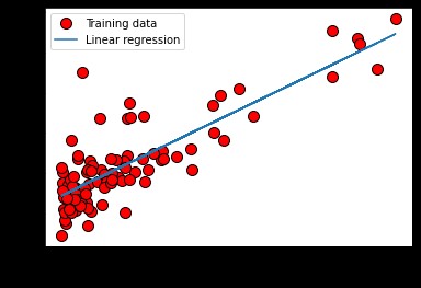
Lets use our learned parameters θj to make food truck profit predictions in areas with a population of 40,000 and 65,000.

print('For population = 40,000, predicted profit = $%.2f' % (predict(4, theta0, theta1)*10000))
print('For population = 65,000, predicted profit = $%.2f' % (predict(6.5, theta0, theta1)*10000))

For population = 40,000, predicted profit = $10351.58
For population = 65,000, predicted profit = $39510.64

That is about it. We can also perform Multivariate Linear Regression, but that is for some other day!

References: